Europe's Debt Has Three Clocks

A government can publish a manageable-looking debt ratio and face a difficult refinancing calendar. Another can carry a much larger debt stock while having more time before higher market rates reach its budget.

The difference is not a statistical curiosity. It is one of the central facts of sovereign finance.

Public debate usually concentrates on how much a country owes relative to the size of its economy. That is a necessary starting point. It does not tell us when the cash must be raised, at what price, or which investors will absorb the securities.

I would read Europe’s new debt figures through three clocks: the stock of obligations, the timetable for funding them, and the gradual arrival of interest costs in the budget.

The clocks interact, but they do not move at the same speed. Confusing them encourages both premature crisis predictions and unjustified reassurance.

What the latest release shows

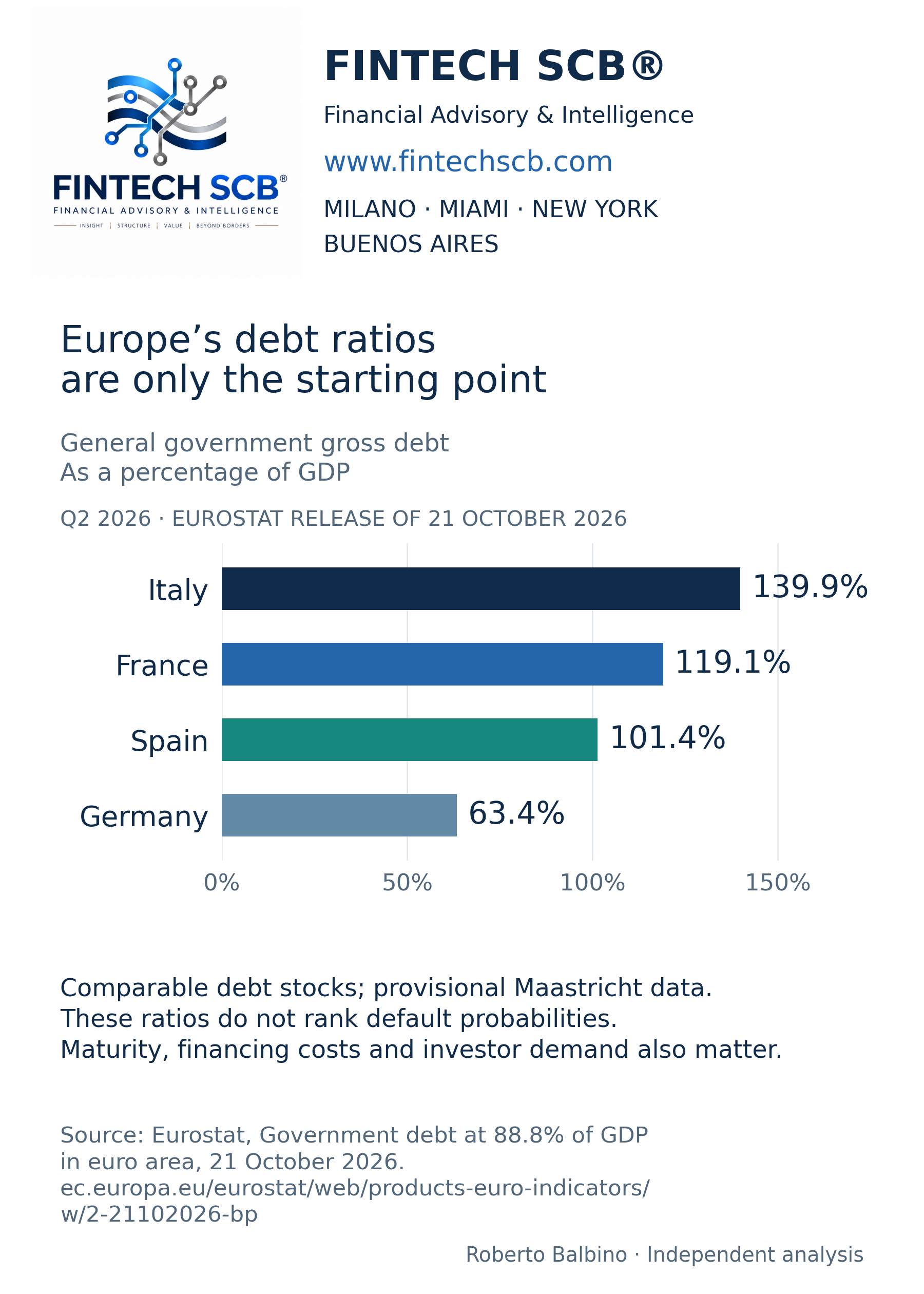
Eurostat’s 21 October release puts euro-area general government gross debt at 88.8% of GDP in the second quarter of 2026, compared with 88.4% in the first quarter. The corresponding country ratios include Italy at 139.9%, France at 119.1%, Spain at 101.4% and Germany at 63.4%. [1]

Debt securities account for 84.5% of the euro-area total. That makes the functioning of bond markets central to financing, although not every security matures or reprices at once.

The chart presents comparable stock measures for the four countries. It does not rank their probability of default. These are provisional Maastricht general-government gross-debt figures, not market values or central-government bond totals alone.

The news is a renewed reason to examine financing structures. It is not, by itself, evidence that a particular country’s next auction will fail.

The first clock: the debt stock

Debt relative to GDP compares a stock of contractual obligations with a flow of national income. The ratio offers a useful measure of scale, but its numerator and denominator can change for different reasons.

A budget deficit usually adds to borrowing needs. Other transactions can affect gross debt too: changes in cash holdings, financial-asset purchases, valuation effects where relevant and differences between cash and accrual accounting.

A government can borrow to build a cash buffer, raising gross debt without an equivalent increase in current spending. It can use that buffer later, reducing the need for immediate market issuance. These choices change the timing of funding even when the underlying fiscal problem is similar.

The GDP denominator also matters. Stronger nominal GDP can reduce the ratio even if the nominal debt stock rises. Weak nominal growth can make stabilisation harder despite measures to control the deficit.

An analyst should therefore ask what drove the movement. A falling ratio associated with durable productive growth is different from one helped temporarily by a price surge. A rising ratio associated with a one-off financial transaction differs from one driven by a persistent primary deficit.

The headline is the entry point to that decomposition, not the conclusion.

The second clock: the funding calendar

A government needs money for new deficits and for obligations reaching maturity, subject to its cash position and other financing operations. The amount it must raise can be much larger than the annual deficit.

Consider a hypothetical country with debt equal to 100% of GDP. If 20% of that stock matures in the coming year and the government also has a cash deficit of 3% of GDP, gross financing needs are approximately 23% of GDP before cash-buffer changes and other adjustments.

A second country with the same debt ratio and deficit, but only 5% of the stock maturing, faces approximately 8% of GDP on the same simplified basis.

Both governments have identical headline debt and deficit ratios. Their exposure to current market conditions is very different.

Debt managers can alter that exposure by choosing maturities, issuance instruments and cash buffers. Longer maturities can buy time, but may carry a higher cost. Shorter funding can appear economical while increasing the frequency with which the issuer must return to the market.

There is no maturity structure that dominates in every environment. The choice involves a trade-off between expected cost and refinancing risk. It should be assessed before a disruption, when time is still available to make adjustments.

The third clock: interest reaches the budget gradually

A rise in the ten-year yield does not immediately reprice every fixed-rate bond already outstanding. The budget typically feels the new rate as debt matures, new deficits are financed or floating-rate and other repricing obligations adjust.

Using the same two illustrative countries, assume newly refinanced debt costs two percentage points more than before. With 20% of a debt stock equal to GDP repricing, the annualised additional interest on that refinanced portion is 0.4% of GDP. With 5% repricing, it is 0.1%.

These are simplified full-year run-rate calculations. Actual first-year cash costs depend on the dates of issuance and payment, instrument design and the cost of financing new deficits. The example does not estimate any named country’s budget.

The important point is the lag. A long maturity profile can delay the adjustment. It cannot permanently remove the cost of repeatedly borrowing at higher rates.

This creates a communication trap. Markets can deteriorate before the annual interest bill rises markedly. Conversely, the budget can continue to absorb higher costs from earlier refinancing even after current yields begin to ease.

The market price and the budget burden are connected through a calendar, not a switch.

France illustrates why definitions matter

Agence France Trésor reports an average maturity of eight years and 158 days for negotiable central-government debt at 30 September 2026. [2]

That is useful information about the financing structure. It is not a statement that nothing matures for eight years. An average can coexist with substantial near-term maturities and a long tail of distant obligations.

It also describes a different perimeter from Eurostat’s general-government gross debt. Central-government negotiable securities do not include every obligation counted in the broader statistical measure. Comparing the two without acknowledging their coverage can create a fictitious inconsistency.

The same discipline applies across countries. A quoted average maturity can refer to all debt, marketable debt, central government or another subset. A meaningful comparison requires matched definitions and dates.

Good sovereign analysis often begins with these unglamorous checks. A sophisticated conclusion built on mismatched measures remains a weak conclusion.

The debt arithmetic behind the politics

A simplified debt-ratio identity is:

Change in debt/GDP = [(r - g) / (1 + g)] × previous debt/GDP - primary surplus/GDP + stock-flow adjustments.

Here, r is the effective nominal interest rate on the relevant debt stock, and g is nominal GDP growth. A primary surplus excludes interest spending. The current benchmark bond yield is not automatically the effective rate r.

For illustration, start with debt equal to 100% of GDP, an effective interest rate of 3%, nominal growth of 4%, no primary balance and no stock-flow adjustment. The ratio declines by approximately 0.96 percentage points through this mechanism.

If the effective rate is 4% and nominal growth 2%, the ratio instead rises by approximately 1.96 percentage points before the primary balance and other adjustments.

Neither calculation is a forecast. It shows why growth, average funding costs and the primary balance must be analysed together.

It also shows why inflation is an unreliable fiscal strategy. An unexpected rise in prices can initially raise nominal income relative to fixed nominal obligations. But financing costs, indexed spending, public wages and other claims can subsequently adjust. The temporary arithmetic gain is not a substitute for a credible fiscal framework.

Who will hold the debt?

For a market price to change, it is not necessary for every existing investor to sell. The terms on which the marginal buyer is willing to add exposure can move yields across the market.

A pension investor matching long liabilities, a bank managing liquidity, a foreign reserve manager and a leveraged trading strategy can all hold government securities for different reasons. Their reactions to price changes and stress need not be the same.

This is why a holder breakdown is useful, but not sufficient. Broad labels conceal leverage, hedging, concentration and investment mandates. “Domestic” is not a synonym for stable; “foreign” is not a synonym for speculative.

The relevant analysis asks how much new supply the market must absorb, how demand responds to yields, whether investors need financing and how resilient market-making capacity remains during volatility.

The debt stock does not answer those questions. A financing strategy must.

The historical change in the central bank’s role

Europe’s sovereign-market architecture has changed through successive episodes. In September 2012, the ECB set out the framework for Outright Monetary Transactions, with conditionality attached to an appropriate assistance programme. The objective included safeguarding monetary transmission. [3]

Large-scale asset purchases later created a different market environment. The ECB’s 2024 annual report records the end of APP reinvestments from July 2023 and the end of PEPP reinvestments at the close of 2024. These dates describe the programmes’ historical change; they are not estimates of today’s country-level financing gap. [4]

The economic implication is that governments and markets cannot assume the same pattern of automatic reinvestment that prevailed in an earlier phase. Other investors must absorb the relevant net supply, at prices that make holding it attractive.

That adjustment can be orderly. Higher yields can draw demand, fiscal plans can improve and issuance can be managed. The existence of a different buyer mix does not establish an imminent liquidity crisis.

It does make the terms of private demand more consequential. Treating the central bank as a permanent buyer at yesterday’s conditions would miss the change in market structure.

Transmission protection has a purpose and conditions

The ECB’s Transmission Protection Instrument, announced in July 2022, addresses unwarranted and disorderly market dynamics that threaten monetary-policy transmission. Its design includes eligibility considerations and a Governing Council assessment. [5]

That is different from a general commitment to validate every fiscal decision or prevent every movement in sovereign spreads. Market conditions and country fundamentals remain relevant.

The distinction matters for both critics and optimists. A currency union needs instruments to prevent destabilising fragmentation from impairing its monetary policy. Governments still need credible fiscal and economic strategies.

Confusing those responsibilities produces bad incentives. Assuming that no support can ever exist exaggerates some crisis narratives. Assuming that support eliminates fiscal constraints understates them.

The institutional framework changes the nature of risk. It does not make debt analysis unnecessary.

Banks and nonbanks connect the fiscal story to markets

Government bonds play several roles simultaneously. They finance the state, serve as investments, support liquidity management and can be used as collateral.

This means a sovereign yield movement can affect financial institutions through more than one route. A bank may experience valuation changes on securities while also facing a different deposit and lending environment. A leveraged investor may face larger margin requirements or more expensive financing. A long-term investor may find new purchases more attractive.

Those effects can offset or reinforce one another. The outcome depends on duration, accounting treatment, hedging, funding and the ability to hold assets through volatility.

An increase in government bond supply also does not mechanically crowd out private investment one for one. Additional securities can satisfy demand for liquid assets. Productive public investment can support private activity. But sustained financing needs can compete for balance-sheet capacity or contribute to higher required returns under some conditions.

The correct question concerns the composition of spending, the response of saving and investment, and the conditions under which the debt is held. A slogan about public borrowing cannot replace those relationships.

Spending quality belongs in debt analysis

A public project that improves transport, energy reliability or human capital can raise future productive capacity. A project selected poorly can leave maintenance costs and debt without an adequate economic benefit.

Even a socially valuable project does not necessarily generate enough additional tax revenue to finance itself. Economic return and fiscal cash return are related but distinct.

That distinction should discipline both austerity and expansion arguments. Cutting a high-return investment can weaken future growth. Borrowing for an inefficient project can weaken the public balance sheet. The category “capital spending” does not determine the quality of a decision.

A credible fiscal strategy explains what is financed, how recurring costs are covered, what assumptions are made about growth and what changes if those assumptions disappoint.

Investors do not need governments to predict the future perfectly. They do need a plausible capacity to respond when the central forecast is wrong.

What would make the outlook better or worse?

The constructive scenario combines stronger productive growth, a credible primary-balance path, manageable maturities and durable investor demand. A high starting debt ratio can then become less burdensome over time, though adjustment remains exposed to shocks.

The adverse scenario combines weak nominal growth, rising effective interest costs, persistent financing needs and political difficulty adjusting revenue or spending. The three clocks then work against the issuer: the stock remains large, maturities keep arriving and the budget absorbs higher costs.

A third scenario is prolonged pressure without a dramatic crisis. Governments retain access to markets but devote more resources to debt service, leaving less room for priorities that voters can see. Fiscal strain can become politically consequential long before an auction fails.

For that reason, I would monitor the maturity calendar, cash buffers, effective funding costs, interest relative to revenue, primary balances, investor composition and the quality of the growth assumption together.

The latest debt ratios justify attention. They do not justify abandoning distinctions. Europe’s fiscal future will be decided by how much it owes, when it must refinance, what it pays and what the borrowed resources help produce.

The debt stock tells us the scale of the obligation. The three clocks tell us how it enters the economy.

Sources and data notes

[1] Eurostat, Government debt at 88.8% of GDP in euro area, 21 October 2026, Q2 2026. EA21 aggregate; provisional general-government gross-debt figures under the Maastricht definition.

https://ec.europa.eu/eurostat/web/products-euro-indicators/w/2-21102026-bp

[2] Agence France Trésor, Negotiable debt outstanding at 30 September 2026. Central-government negotiable-debt perimeter; distinct from Eurostat general-government gross debt.

https://www.aft.gouv.fr/en/node/452

[3] ECB, Governing Council decisions, September 2012, including the OMT framework announced on 6 September 2012. Historical institutional context.

https://www.ecb.europa.eu/press/govcdec/otherdec/2012/html/gc120921.en.html

[4] ECB, Annual Report 2024, asset-purchase and reinvestment developments. Historical context; no current country-level buyer shares are inferred.

https://www.ecb.europa.eu/pub/pdf/annrep/ecb.ar2024~8402d8191f.en.pdf

[5] ECB, The Transmission Protection Instrument, 21 July 2022. Instrument design, eligibility and activation principles.

https://www.ecb.europa.eu/press/pr/date/2022/html/ecb.pr220721~973e6e7273.en.html

Refinancing and debt-dynamics examples are Fintech SCB illustrations, not country forecasts. The two-percentage-point shock is applied only to the assumed refinanced stock. Debt/GDP alone is not used as a measure of default probability.

Roberto Balbino — Founder & CEO, Fintech SCB

Independent analysis of finance, economics, geopolitics and global markets

www.fintechscb.com

#PublicDebt #Eurozone #BondMarkets #FiscalPolicy #Banking #Macroeconomics #RobertoBalbino #FintechSCB