MID TRUMP

Roberto Balbino | FINTECH SCB

Sunday, November 1, 2026

A president does not set the world’s prices. But a president can change the conditions under which the world prices almost everything.

A tariff changes the cost of bringing a product into a country. A military operation changes the probability that a tanker reaches its destination. A tax law changes the government’s future borrowing requirements. An immigration decision changes the supply of workers. A nomination changes who sets the cost of money. A regulatory decision changes which financial products can exist, which institutions can hold them and how much investors are willing to pay for them.

Donald Trump’s second presidency has operated through every one of these channels, often at the same time.

The consequences appear in places that do not look political: a German manufacturer’s energy bill, an American mortgage application, a Brazilian company’s dollar funding, a Japanese importer’s working capital, a Bitcoin liquidation, the discount rate used to value a data centre, the refund cheque that a customs broker is now chasing on behalf of a client.

This is the economic meaning of MID TRUMP.

The United States is approaching the midpoint of a presidential term that began on January 20, 2025. Strictly speaking, the period under examination is twenty-one months, not two completed years. It has been long enough for the major decisions to move from announcements into prices, contracts, investment plans and public finances. It has not been long enough for all of them to finish passing through.

The central question is how much of the present economic environment can reasonably be traced to those decisions.

Answering it requires more discipline than placing an inauguration date on a market chart. Something that happened under Trump was not necessarily caused by Trump. A policy can have a measurable effect without explaining an entire market movement. And the same administration can introduce measures that push the same price in opposite directions.

The useful exercise is to follow the transmission: decision, mechanism, evidence, distribution of the cost, and future exposure.

What emerges is a presidency that has altered several of the world’s most important prices simultaneously, and created interactions between them that are more consequential than any individual announcement.

THE STANDARD OF EVIDENCE

Before the numbers, the rules of the exercise.

The strongest attribution combines a clearly identified decision, a plausible mechanism and evidence that more exposed goods, firms or countries behaved differently from less exposed ones. The tariff estimates published by the Federal Reserve meet that standard.

The next level is documented physical or financial transmission: a military decision, followed by shut-in production, followed by higher insurance and freight, followed by prices. The energy shock of 2026 meets that standard.

The weakest attribution is an aggregate asset price that moved over a long period in which many things changed. A stock index, Bitcoin, the dollar or the ten-year yield since inauguration belongs in a description of the period. None of them is, on its own, a measure of the president’s economic contribution.

A rigorous assessment should therefore be willing to reach conclusions of different strength. Some effects can be estimated. Some can be traced but not precisely quantified. Others remain hypotheses. This is not an obstacle to a forceful argument. It is what makes the argument credible.

INFLATION: THE INHERITED LEVEL AND THE POLICY ADDITION

The United States entered this administration with an elevated price level inherited from the pandemic and its aftermath. A lower inflation rate does not restore the previous price level. It means prices are rising more slowly. A government can therefore inherit widespread dissatisfaction with the cost of living even while the inflation rate is declining.

But an inherited problem and an additional, policy-induced problem can coexist. Both are visible in the data.

The last consumer-price release before the election, published by the Bureau of Labor Statistics on October 14, shows annual inflation of 3.7% in September 2026, with prices rising 0.6% in the month. The core measure, excluding food and energy, rose 2.6% over the year. Energy prices were 20.4% higher than a year earlier and gasoline 34.2% higher. Gasoline alone accounted for more than half of September’s monthly increase.

Two further numbers complete the picture. The consumer price index was 6.1% higher in September 2026 than in January 2025, the month of the inauguration. And average hourly earnings rose 3.0% over the twelve months to September, below the 3.7% rise in prices. In the latest data, real pay is falling.

Three phases are visible. Inflation drifted down from 3.0% in January 2025 to a low of 2.4% in February 2026. It then rose to 4.3% in May, after the start of the war, before settling between 3.4% and 3.7% through the summer and early autumn. The first phase is mostly inheritance and disinflation; the second is energy; the tariff effect sits underneath both.

Figure 3. Inflation: tariffs first, then energy (Fintech SCB; data: BLS, Federal Reserve)

For attribution, the tariff evidence is particularly useful.

A Federal Reserve research note published on April 8, 2026 estimated that the tariff changes implemented between February and November 2025 had raised core goods PCE prices by 3.1% through February 2026, contributing about 0.8% to the level of overall core PCE prices. The authors found that the effects accumulated over time and that pass-through was effectively complete within the period they studied. They attribute to tariffs essentially all of the excess core goods inflation relative to pre-pandemic rates, and they explicitly exclude the tariff changes that followed the February 2026 Supreme Court ruling.

That is a much stronger statement than observing that inflation rose during the presidency. It identifies a specific intervention, compares differently exposed goods and estimates the resulting price effect. It also establishes limits: particular tariffs, a particular period, a particular inflation measure, first-round effects only. A cumulative increase in the price level is not a permanent annual increase in inflation of the same magnitude.

The economics behind the finding are simple.

A tariff is collected from the importer. The ultimate burden is then distributed among foreign suppliers, importers, retailers, workers and consumers. A foreign producer might accept a lower price. A distributor might absorb part of the cost through a smaller margin. A retailer might eventually raise the shelf price. The distribution depends on competition, exchange rates, substitution, inventories and negotiating power. There is no economic rule under which the foreign country automatically pays the bill, and the Fed’s estimate indicates that in 2025 the American buyer paid most of it.

There is also no requirement that the bill arrive immediately. Goods imported before a tariff increase can remain in warehouses for months. Firms can protect customers at first, then adjust prices when replacement inventory becomes more expensive. Temporary margin compression precedes consumer inflation. This delay explains why the economic effects of a decision outlast the news cycle that produced it.

The impact extends beyond imported finished goods. A domestic manufacturer using imported machinery, metals or components faces higher costs even when its final product is made in America. Protection for one industry becomes an input cost for another. The relevant financial question for any company is therefore how its protection compares with its exposure, evaluated at the level of its actual production and sales structure.

For households, the analogous question is which goods became more expensive relative to their incomes. The same aggregate inflation rate produces very different experiences across families.

For the rest of the world, the transmission is more complicated. American tariffs divert goods toward other markets, which can lower prices there. They weaken demand for the exports of trading partners. Both channels can be disinflationary outside the United States. At the same time, reorganising supply chains raises costs, retaliation raises local prices, and exchange-rate movements amplify or offset the original shock. It would be analytically wrong to describe every tariff as inflationary everywhere.

TARIFFS AFTER THE COURT: THE PRICE STAYED, THE REVENUE IS GOING BACK

The tariff story changed legal shape in 2026, and the change matters for anyone trying to assign costs.

On February 20, 2026, the Supreme Court held in Learning Resources v. Trump that the International Emergency Economic Powers Act does not authorise the president to impose tariffs. The reciprocal and trafficking tariffs of 2025 were unlawful from the start. The administration replaced them within days with a 10% global tariff under Section 122 of the Trade Act, later raised to 15%, which by law expired after 150 days on July 24. It was then replaced by Section 301 tariffs of 10% or 12.5% on imports from about sixty economies, with product exemptions. The Section 232 tariffs on steel, aluminium and vehicles, which rest on a different statute, were never affected.

Two consequences follow.

First, the average effective tariff rate fell but did not return to where it started. The Penn Wharton Budget Model calculates that customs duties as a share of import value rose from 2.3% in January 2025 to 7.1% in August 2026, the first full month under the Section 301 regime, or 10.1% had imports followed their historical pattern instead of shifting toward exempt goods and USMCA-qualified trade. The Congressional Budget Office puts the current effective rate at about 10%, five percentage points below its November 2025 estimate.

Second, the money collected under the struck-down tariffs is being refunded. About $166 billion of IEEPA duties were collected before the ruling. By October 2, Customs had certified about $126 billion for refund, with interest. Refunds began in May; in some months they came close to offsetting new customs receipts.

Here is the distributional point that most commentary misses. The refund goes to the importer of record. The price increase, according to the Fed’s own estimate, was passed through to the consumer. Unless downstream contracts force importers to share the money, which some do and most do not, the 2025 tariffs end up as a transfer from American shoppers to the companies that paid the duty at the border and then recovered it from both the customer and the Treasury.

Figure 5. Fiscal: the tariff money the budget counted on is going back (Fintech SCB; data: CBO, Penn Wharton Budget Model)

This also rewrites the fiscal arithmetic, to which we return below.

ENERGY: THE PRICE OF A MILITARY DECISION

The more important global inflation channel in 2026 has been energy.

On February 28, Trump announced that the United States had begun major combat operations in Iran, in a joint operation with Israel. The decision to undertake those operations is directly attributable to the administration. The subsequent course of the conflict involves other actors, decisions and contingencies. That distinction does not weaken the economic connection. It makes it more precise.

The causal chain runs from military escalation to risks affecting production, export infrastructure and shipping; from those risks to physical shortages and higher transport costs; and from energy costs to inflation, corporate margins and monetary-policy expectations.

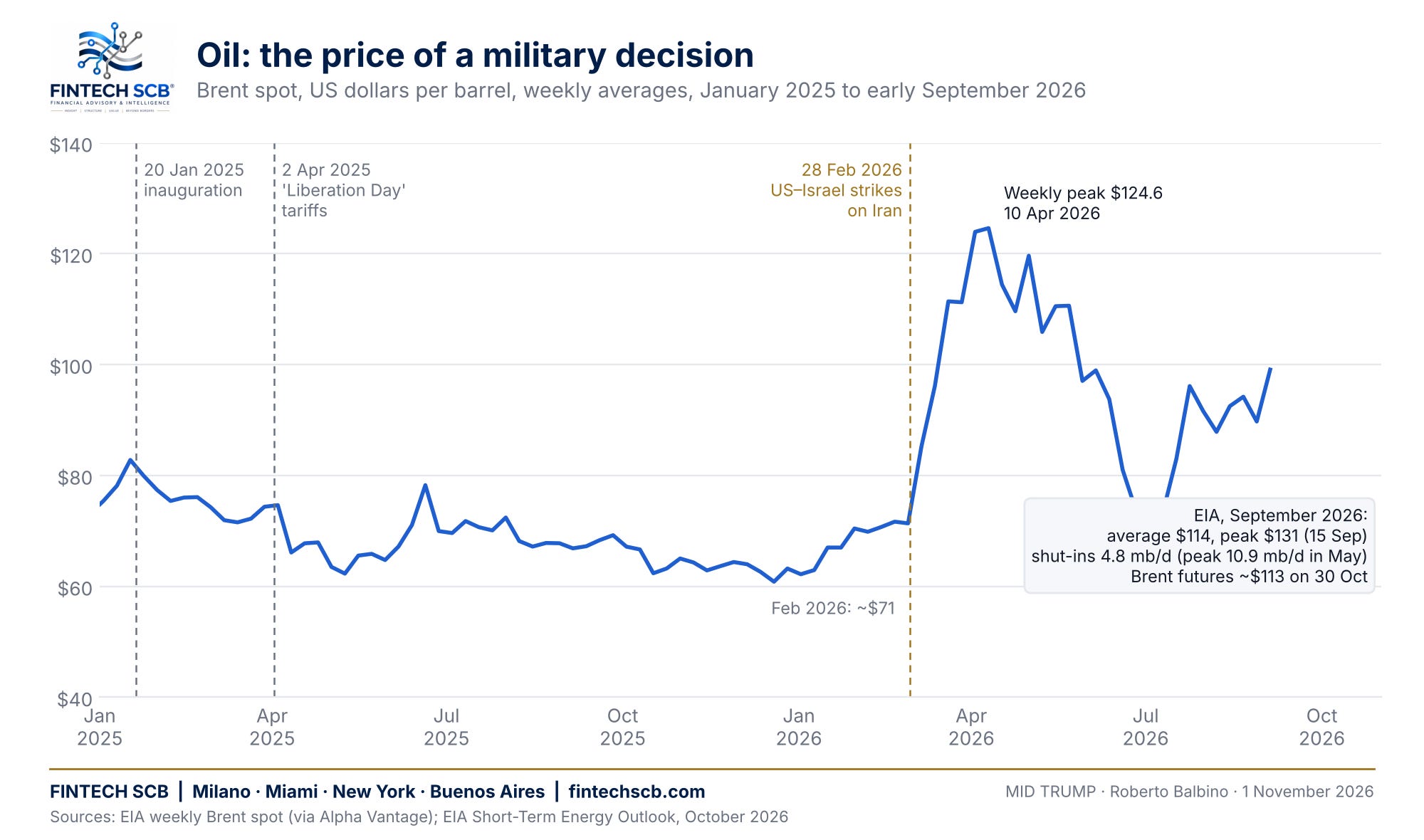
The Energy Information Administration’s October outlook describes the disruption concretely. Brent spot averaged $114 a barrel in September, $23 above August, after attacks on Middle Eastern oil infrastructure and tankers, including Saudi Arabia’s East-West pipeline, the bypass that avoids the Strait of Hormuz. Daily Brent reached $131 on September 15. Production shut-ins averaged 4.8 million barrels a day in September, down from a peak of 10.9 million in May. Tanker rates reached record levels on higher insurance costs, ships took longer routes, and global inventories fell by an average of 1.9 million barrels a day in the third quarter. Brent futures closed at about $113 on October 30.

Before the war, Brent had averaged about $71 in February 2026. Weekly averages peaked near $125 in April.

Figure 1. Oil: the price of a military decision (Fintech SCB; data: EIA)

This is a shock with several components. The oil itself becomes more expensive. Transport becomes more expensive. Insurance becomes more expensive. Delivery becomes slower and less reliable. Refiners may have to replace a preferred crude with a less suitable one. The cost of a usable barrel delivered to a refinery therefore moves differently from the headline benchmark, which is why “the oil price” is a poor single number for financial analysis.

For an airline, jet-fuel availability and refining margins matter. For a trucking company, diesel. For a manufacturer, electricity, natural gas, petrochemical inputs or freight. For a farmer, fuel and fertiliser. A crude shock does not move through every industry at the same speed.

Nor does higher American production insulate American consumers. Oil is traded internationally; producers sell into the best available market; refineries differ in the grades they can process. Additional domestic output improves supply and the trade balance without making domestic fuel prices independent of global conditions. And there is a timing problem: permitting, financing, building and bringing production online are different events. A policy that may expand supply over several years cannot offset a disruption occurring this month.

This is one of the central tensions of the presidency. Measures intended to improve domestic energy supply over time operate alongside a foreign-policy decision that raised energy costs immediately. American gasoline up 34.2% in a year is the domestic receipt for that tension.

The impact abroad is larger.

On October 29, the European Central Bank held its rates and reported euro-area inflation of 3.8% in September, with energy inflation at 18.9%. It said the increased magnitude and duration of the energy shock were likely to raise inflation and lower growth, including through second-round effects. It also noted that underlying inflation had remained broadly stable and that wages did not yet show a material response. Those observations distinguish imported energy pressure from a domestic wage-price spiral. The ECB had already raised rates in June and September to meet a shock it did not cause.

For Europe, the problem is not simply a larger fuel bill. More income must be transferred to energy suppliers to obtain the same physical quantities. A government can cushion the transfer through subsidies or tax cuts, but the cost then appears in public finances. A company can absorb it through margins, but the cost then appears in profits and investment. A household can absorb it through reduced consumption elsewhere. The burden changes location. It does not disappear.

One partial offset deserves mention. The dollar has weakened: the euro bought $1.04 on inauguration day and about $1.12 at the end of October. For a European importer, a barrel priced in dollars costs fewer euros than the dollar price alone implies. That cushion is real but small against a price that nearly doubled.

The International Monetary Fund’s October outlook projects global growth of 3.1% in 2026 and global headline inflation of 4.7%, up from 4.1% in 2025. It assumes an average oil price of $95.74 for the year, 41% above 2025, and links the slowdown in the euro area and China to energy. It also flags, in the same report, that a reassessment of expected returns from concentrated AI investment could trigger financial corrections. Those are forecasts, not outcomes.

The distribution matters more than the global average. An energy exporter receives a windfall. An importer sees its external balance deteriorate. A country with large dollar debts faces an additional burden if its currency weakens. A government with limited fiscal space has fewer options. The same American decision generates different outcomes across countries without any inconsistency in the analysis.

THE PRICE OF MONEY: THE FED CUT, THE BOND MARKET DID NOT

A government bond is a claim on future nominal payments. Its price depends on the return investors require to hold those payments over time. When required yields rise, the price of an existing bond falls. But the reason yields rise matters.

Investors may expect stronger real growth, higher inflation, higher policy rates, more compensation for holding long maturities, or more debt than intermediaries can comfortably absorb. Trump’s decisions touch several of these at once: tariffs and energy affect inflation expectations and the policy path; tax and spending legislation affects borrowing requirements; the choice of a Federal Reserve chair affects the reaction function; policy uncertainty affects the premium investors demand for committing capital.

The sequence of the last twenty-one months is instructive.

The Federal Reserve held its policy rate at 4.25–4.50% through the first eight months of 2025, then cut three times between September and December to 3.50–3.75%. Trump nominated Kevin Warsh as chair on January 30, 2026; he was sworn in on May 22. In September 2026, with headline inflation back above 3.5%, the Fed raised rates for the first time since 2023, to 3.75–4.00%. On October 28, six days before the election, it held, with two members voting for a further increase.

The bond market moved further and earlier. The ten-year Treasury yield, which had fallen to about 4.0% in February 2026, climbed to 5.26% in early October, a level not seen since 2007, before easing to 4.94% on October 30. The thirty-year closed that day at 5.31%. The national debt passed $40 trillion.

Figure 2. Money: the Fed cut, the bond market did not (Fintech SCB; data: US Treasury, Federal Reserve)

An elementary illustration shows the sensitivity. A bond portfolio with a modified duration of eight years loses about 8% for a one-point rise in yields, before convexity. That is a financial approximation, not an estimate of losses caused by Trump. Its relevance is that modest changes in required returns produce large changes in asset values, and the same repricing reaches borrowers: mortgage rates, corporate yields and project-finance costs sit on top of government yields.

A decision taken in Washington can therefore determine whether a business expansion in another country still clears its investment hurdle.

The last fortnight shows why bond moves need care. The Financial Times reported on October 31 that investors were cutting growth expectations as concerns about the AI investment cycle increased, buying government bonds and pushing the ten-year inflation-protected yield down to 2.58%, its lowest since early September. That is a rally driven by fear of weaker growth, not by confidence in fiscal discipline. Bond prices can rise because growth is expected to slow or because inflation risk is falling. The same market direction carries different information. A political reading that celebrates every bond rally and condemns every sell-off will misread the evidence repeatedly.

The more interesting possibility is that policy has created competing forces: pressure on inflation and financing costs on one side, concern about the durability of growth on the other. The balance between them changes with each data release.

FISCAL POLICY: WHAT THE DECISIONS ADD TO THE DEBT

The Congressional Budget Office’s outlook of February 11, 2026 estimated that the 2025 reconciliation act adds $4.7 trillion to deficits over 2026–2035, including $0.9 trillion in debt service. It estimated that higher tariffs reduce deficits by about $3 trillion over the same window, and that lower immigration increases them by $0.5 trillion. It projected a 2026 deficit of $1.9 trillion, or 5.8% of GDP, and debt at 120% of GDP in 2036, with net interest rising from $1.0 trillion to $2.1 trillion a year.

Nine days later the Supreme Court removed the legal basis of most of the tariffs in that baseline.

In its August 20 update, the CBO estimated that the trade-policy changes through July 31, including the refund of most of the $166 billion collected under IEEPA, make deficits $0.9 trillion larger over 2027–2036 than its February projection, and cut projected net customs revenue for fiscal 2026 by $250 billion.

The figures illustrate why fiscal analysis must consider the package. A tax cut raises private investment incentives while lowering revenue. A tariff raises revenue while raising private costs. Lower immigration reduces some spending while reducing employment, output and receipts. A court ruling can erase a revenue line while leaving the price effect in the shops. There is no contradiction in a policy producing a benefit in one account and a cost in another, and no contradiction in the same tariff producing a cost for consumers, a gain for the Treasury, and then a refund that reverses only the second.

Nor should the increase in total debt be attributed entirely to this administration. Existing law, ageing, inherited debt, interest rates and the cycle all contribute. The useful question is what the new decisions add relative to a clearly specified baseline. Net of the four items above, the answer is roughly $3 trillion over ten years, before the cost of financing it at the yields the market now requires.

For investors, the timing of refinancing matters as much as the stock of debt. Higher yields do not reprice every outstanding Treasury at once. The burden builds as debt rolls over and new deficits are financed. This creates a lag between a market shock and its full budgetary effect, and a potential feedback loop: more borrowing, higher interest, more borrowing to pay the interest, and greater sensitivity to the next refinancing cycle. The loop is not automatic; growth, revenue, spending adjustments and investor demand can interrupt it. But it is a meaningful exposure, and the Treasury’s refunding announcement on Wednesday, the day after the vote, is the next data point on it.

ARTIFICIAL INTELLIGENCE: GROWTH THAT ARRIVES BEFORE THE RETURN

The administration did not invent the AI investment cycle. Private research, corporate competition, semiconductor development and earlier investment decisions preceded it. Trump did, however, make identifiable decisions to accelerate its physical infrastructure. The executive order of July 23, 2025 directed federal agencies to speed permitting for data centres, identify federal sites and explore financial support, including for the power and transmission infrastructure that the facilities need.

Faster permitting has real economic value. For a project that earns revenue only when construction is complete, a shorter development period reduces financing costs and brings cash flows forward. More predictable approvals reduce the uncertainty that investors price into a project.

But faster approval does not guarantee sufficient power, customer demand or an adequate return on capital. An AI facility consumes scarce resources before it generates productivity gains elsewhere: equipment, construction labour, land, grid connections and finance. When many projects require the same resources at the same time, the boom raises their prices. A technology can be disinflationary over a decade and inflationary for particular inputs over the next two years.

The last week illustrated the financial side of that timing. Alphabet reported quarterly capital expenditure of $51.4 billion, above its operating cash flow, and a second consecutive quarter of negative free cash flow; its shares fell 13% in a day. The Nasdaq 100 fell into correction territory. Third-quarter GDP grew at an annualised 3.4%, with investment, including AI hardware, providing most of the contribution. For the statistician, capital spending is growth. For the shareholder, it is cash out of the door before the profitability of the asset is known.

This is why the measured economy and the market can diverge in opposite directions at the same time. PGIM’s chief US economist told the FT that his recession probability had risen from 10% early in the year to perhaps 25%, while the probability of strong growth had also risen: fatter tails on both sides, driven by one sector.

The presidency influences this environment through permitting, taxes, trade restrictions and energy policy. It cannot be assigned responsibility for every corporate capital-allocation decision. Yet the channels interact. An administration can make a data centre easier to approve while making imported equipment more expensive. It can improve after-tax investment incentives while contributing to conditions that raise the cost of borrowing. It can encourage an electricity-intensive industry while other policies increase energy-market volatility.

A policy package should be assessed for internal economic consistency, not merely for the stated objective of each component.

One further point from the FT’s election guide: two of the largest data-centre hubs, Texas and Ohio, have tight governors’ races, and fund managers interviewed by the paper said the gubernatorial outcomes could matter more for the AI build-out than Congress, because permitting, land and power are decided in state capitals. The presidency opened the federal door. The states hold the keys to the grid.

CRYPTO: REGULATORY SUPPORT, MACRO HEADWINDS

Cryptocurrency offers an unusually clear illustration of competing presidential effects.

Trump took measures that directly support the institutional development of digital assets. The executive order of March 6, 2025 established a Strategic Bitcoin Reserve, capitalised with forfeited government holdings and permitting further acquisition only on a budget-neutral basis. That is different from an unrestricted commitment to buy Bitcoin in the market: retaining an existing asset reduces expected future selling; buying creates fresh demand. Both affect expectations, but they are not the same flow. In July 2025 he signed the GENIUS Act, a federal framework for payment stablecoins with full reserve backing in liquid assets and public disclosure.

Regulatory clarity lowers uncertainty, encourages infrastructure investment and widens the range of institutions willing to participate. Those are real channels of support.

But crypto prices also respond to the cost of money, leverage and risk appetite. Bitcoin traded near $101,000 in the week of the inauguration, reached a weekly closing peak of $123,500 on October 5, 2025, and then fell. The record liquidation of October 10, 2025 followed a new tariff threat against China. Further selling followed the Warsh nomination in January 2026, on expectations of a tighter liquidity environment, and the start of the war. The weekly low was $59,500 at the end of June 2026. On November 1 the price is about $77,500: roughly a quarter below the inauguration week, after a presidency that has been more favourable to the sector than any before it.

Figure 4. Crypto: regulatory support, macro headwinds (Fintech SCB; data: Alpha Vantage)

Regulatory friendliness does not suspend financial arithmetic. When safe assets pay 4% or 5%, speculative assets compete against a different opportunity cost. When leveraged investors face margin calls, assets are sold because they are liquid, regardless of the thesis attached to them. A favourable speech cannot prevent a forced liquidation.

Stablecoins reveal a connection that is often missed: part of the digital-asset ecosystem supports demand for government debt. Issuers hold short-term dollar assets against their liabilities and become Treasury-bill buyers as they grow. Research published by the Bank for International Settlements finds a measurable relationship between stablecoin inflows and short-term Treasury yields, concentrated at short maturities rather than along the curve.

This creates a distinction within “crypto”. Bitcoin has no contractual dollar value. A dollar stablecoin is built around one. One attracts investors seeking an alternative monetary asset; the other extends the practical reach of the dollar. A policy that promotes dollar stablecoins reinforces dollar-denominated finance even when the public conversation presents crypto as an escape from it.

It is not, however, a solution to the fiscal problem. Some stablecoin purchases are money moving out of other vehicles that already held bills. Gross purchases are not net new demand. And demand for bills does not finance a growing supply of long bonds at unchanged yields, which is where the pressure now sits.

THE DOLLAR: A PRICE THAT RESISTS SIMPLE READINGS

Higher American rates support the dollar by improving the relative return on dollar assets. Stronger growth attracts capital. Global stress raises demand for dollar liquidity. Other forces work the other way: concerns about policy predictability, changing hedging behaviour, diversification, or a deterioration in expected returns.

Over this presidency the second set has dominated against the euro: from $1.04 to about $1.12, a depreciation of roughly 7%, despite American yields well above European ones. A tariff announcement does not contain a mechanically determined exchange-rate outcome.

For foreign borrowers, the combination is what counts. A company earning local currency but servicing dollar debt is exposed to both the dollar interest rate and the exchange rate. A weaker dollar has helped on one leg this year; higher dollar rates have hurt on the other. For importers of energy, a higher dollar oil price combined with their own currency’s weakness produces a larger local-currency increase. This is one reason American decisions have disproportionate effects in economies that have no vote on them.

LABOUR AND IMMIGRATION: THE SUPPLY SIDE

Immigration policy belongs in the same analysis because it changes the supply side of the economy. The effects depend on who enters, who leaves, their skills, their employment, their consumption and the capacity of local infrastructure. Reducing immigration reduces some demand. It also reduces labour supply, and the effects are largest where workers complement existing capital and other employees: a shortage in one trade can stall an entire project rather than merely raise the wage of a direct substitute.

Construction illustrates the mechanism. If a project lacks enough workers to finish on schedule, the consequences include higher labour costs, longer financing periods and delayed housing supply. The full outcome depends on whether firms can recruit other workers, raise productivity, change technology or cut activity. It cannot be read from a single unemployment rate.

The September employment report shows an economy with low unemployment and little dynamism. Payrolls rose 29,000 in the month, against an average of 45,000 over the previous twelve; total employment is up 496,000, or 0.3%, over the year. The unemployment rate is 4.2%. Manufacturing employment fell through 2025 and has recovered 72,000 jobs since its December low. The October Beige Book reports shortages of specialised, technical and skilled-trade workers alongside firms that have reduced staff through attrition or delayed hiring after investing in AI. These are observed outcomes with many causes, not a clean experiment on one policy. The CBO’s $0.5 trillion estimate is the fiscal expression of the same supply constraint.

That distinction should run through the whole assessment. If manufacturing investment rises, the questions are whether projects are completed, how productive they are and whether their gains exceed the costs imposed elsewhere. If employment rises in a protected industry, the analysis must include its customers and downstream producers. If imports fall, one must ask whether domestic production replaced them, demand weakened, inventories changed or trade was rerouted. A smaller trade deficit is not automatically evidence of strength; a larger one is not automatically evidence of weakness.

UNCERTAINTY AS A COST

Another cost deserves more attention: uncertainty about the rules themselves.

A business contemplating a factory must form expectations about tariffs, taxes, labour, energy and market access over many years. When those expectations change repeatedly, waiting becomes valuable. This is the logic of investment under uncertainty: a project can have a positive expected value and still be delayed because committing capital is hard to reverse. In 2025–2026 the rules changed by announcement, by court ruling, by statutory expiry and by replacement, within eighteen months.

An IMF working paper on the 2025 trade shocks used firm-level event analysis to separate exposure to trade from sensitivity to uncertainty, and found that both contributed to valuation changes around tariff announcements and subsequent easing. Investors price the predictability of the rules, not only the rules.

There is a practical corporate-finance consequence. Companies hold more liquidity, duplicate suppliers, shorten contracts or pay for resilience. Those choices can be rational for the firm while lowering aggregate efficiency. Suppose a company consumes $1 million of imported inputs a month and decides to hold one more month of inventory because trade rules or shipping routes have become less predictable. It must finance $1 million more of stock. At 8%, that precaution costs $80,000 a year before warehousing, insurance and obsolescence. The company may rationally conclude that this is cheaper than a production stoppage. The capital is still absorbed.

Research published by the Federal Reserve identifies the competing credit responses to supply-chain uncertainty: firms may postpone investment and borrow less, or borrow more to build inventories and manage disruption, while banks tighten as risks rise. The direction of total borrowing alone does not reveal whether the economy has become healthier. A rise in credit can finance confidence. It can also finance defensive adaptation.

ONE BALANCE SHEET AT A TIME

The transmission becomes clearer when we move from national statistics to the accounts of an individual company.

Consider an importer with $10 million in sales, $1 million in operating earnings and $5 million of debt. Higher financing costs add two percentage points to its interest rate at refinancing: an extra $100,000 a year, equal to 10% of its original operating earnings. Now suppose tariffs, freight and energy reduce operating earnings by another $100,000 because the company cannot pass every increase to its customers. Its debt-to-operating-earnings ratio rises from five times to about 5.6 times without borrowing another dollar. The firm has suffered three changes: lower earnings, higher interest and weaker credit metrics. Its next lender will demand a higher spread precisely because the first two changes have made it riskier.

These are illustrative calculations, not measurements of a particular company. They show why the consequences of policy become nonlinear. The original cost increase may be manageable. Its interaction with leverage is not.

The Federal Reserve’s October Beige Book describes this process in the language of businesses themselves. Higher oil prices affected all twelve districts. Firms reported elevated diesel costs and fuel surcharges passing through supply chains. Consumer-facing businesses reported tighter margins because price-sensitive customers resisted further increases. Several districts expected additional price increases as contracts expire and hedges are renegotiated. Contacts cited continued pressure from tariffs and insurance, and persistent uncertainty around energy and tariffs weighing on the outlook.

The expiry of contracts is the point. A company that fixed its freight before the energy shock appears unaffected. A business with hedged fuel reports stable costs for several quarters. A retailer still sells inventory bought under the earlier tariff regime. When those protections expire, the new economics arrive. The absence of an immediate response does not prove a policy had no effect, and a price increase months later cannot automatically be assigned to the most recent announcement. The exposure must be traced through purchasing dates, inventory turnover, contract terms and hedges.

This makes the period after the election economically consequential even if no dramatic new policy is announced. Some decisions already taken have not finished passing through the system.

INVESTMENT: ANNOUNCEMENTS, ACQUISITIONS AND FACTORIES

Investment announcements have become a prominent feature of the administration’s economic narrative. They deserve examination because credible commitments affect suppliers, employment expectations and infrastructure planning.

But an announcement, an acquisition and a completed factory are different economic events. An acquisition transfers ownership of an existing asset. A new facility expands capacity if it is completed and operated. A multiyear commitment may include projects already planned, contingent on conditions or dependent on future demand.

A Federal Reserve research note of June 26, 2026 found that aggregate foreign direct investment into the United States remained resilient in 2025, with limited visible aggregate effects from tariffs and trade uncertainty, substantial differences between manufacturing industries, and a surge in announced foreign acquisitions concentrated in the AI boom and related technology firms, with completion an open question.

That finding matters for balance. It would be wrong to claim that the administration’s policies drove foreign investors away. It would be equally wrong to treat every announced dollar as proof that tariffs rebuilt manufacturing. America continued to attract capital; the composition of that attraction is what determines its durability. A country remains attractive because of technology, market size, legal infrastructure and industrial clusters even when investors dislike particular policies. Attribution requires asking what changed at the margin: did a tariff induce a producer to build domestically, did tax treatment improve the return, did permitting shorten construction, or would the investment have happened because demand for computing capacity was expanding regardless?

There are also real potential benefits that should be assessed on the same standard as the costs. A simpler approval process reduces delays. Favourable tax treatment of investment improves the return on an additional machine. A credible trade agreement reduces uncertainty after confrontation. A domestic producer gains customers when imports become dearer. The Richmond Fed’s August Beige Book recorded both sides: manufacturers unable to pass on costs, freezing wages or pausing capital spending, and others reporting stronger demand as customers shifted to domestic products.

The central test is whether the benefits are additional, durable and larger than the costs. A factory attracted by protection may build valuable capabilities. If it depends indefinitely on expensive inputs and higher customer prices, its contribution must be weighed against those burdens. A project viable because approvals are faster is a different economic case from one viable only because competitors have been made more expensive. Both raise domestic production. Their effects on productivity and national purchasing power are not the same.

AGRICULTURE: INCOME SUPPORTED, BUSINESS WEAKER

Farms operate between global commodity markets and domestic cost structures. They buy fuel, fertiliser, machinery and finance and sell products whose prices are set internationally. Trade measures alter access to export customers; energy disruptions raise input and transport costs; exchange rates shift competitiveness; government payments cushion the result.

The USDA’s September forecast projects 2026 production expenses of $492.8 billion, up $21.2 billion or 4.5%, with fertiliser up 15.3% and fuel up 28.8%. Cash receipts are forecast at $540.3 billion, slightly lower than 2025. Net farm income falls 2.6% in nominal terms and 5.5% after inflation, to $158.4 billion. Direct government payments rise 69.8% to a record $47.4 billion, of which $26.5 billion is supplemental or ad hoc assistance, including the Farmer Bridge Assistance Program.

Roughly thirty cents of every dollar of net farm income this year comes from the government. The analytical lesson is that farm income can be supported while the underlying business deteriorates. An income figure that includes transfers answers a different question from the profitability of selling crops at market prices. If the government cushions a loss, the burden moves from the producer to the public budget. That may be justified by the policy’s objectives. It is still a transfer that must be counted, and it must be counted against the tariff revenue that was supposed to pay for it and is now being refunded.

Internationally, the effects can change direction. A foreign exporter gains customers who reduce purchases from the United States, and simultaneously pays more for fertiliser, fuel and shipping. Higher volumes do not guarantee higher margins. Commodity economies can benefit from trade diversion while suffering from the energy and financing consequences of the same policy environment.

THE REST OF THE WORLD HAS NO SINGLE BALANCE SHEET

Canada, Mexico and China face a different combination because of their direct integration with American demand. The IMF’s 2026 assessment identified these large trading partners as particularly exposed to the spillovers of the 2025 policy changes; it also discussed countries dependent on migration and remittances, and the possibility that wider use of dollar stablecoins could encourage dollarisation or ease capital outflows in vulnerable economies. These were model-based assessments at the time, not measurements of the full outcome.

For Mexico, the mechanism is manufacturing integration and the terms on which goods cross the border. For Canada, integrated production and commodities. For China, market access, substitution and the redirection of exports. In each case the effective burden depends on actual tariff treatment, exemptions and rules of origin: in August 2026, 81% of imports from Canada and Mexico entered under the USMCA exemption. A headline rate applied to a whole country is a poor measure of what a particular company pays.

For Central American and Caribbean economies, migration policy creates a separate external exposure. Remittances are household income arriving from abroad. Changes in the ability to work in the United States affect those flows, with size and timing depending on employment, enforcement and the channels used. A policy whose domestic objective concerns the American labour market therefore affects consumption, housing and foreign-exchange availability elsewhere.

For Europe, energy dependence combines with industrial competition and financing costs. For many emerging economies, the critical combination is imported energy and dollar liabilities. For energy exporters, higher prices improve public revenues while raising geopolitical and transport risks.

Defence adds a further channel. The June 2025 Hague declaration committed NATO allies to 5% of GDP by 2035 for core defence and related security spending, at least 3.5% for defence proper and up to 1.5% for broader security, with a review in 2029. This is a future commitment with national implementation paths, shaped by the security environment; assigning its entire origin to one president would be unjustified. But its economics belong here. Higher defence spending supports manufacturing, engineering, software and logistics. The fiscal consequence depends on whether it is financed by taxes, by cutting other spending or by borrowing. The industrial consequence depends on procurement: purchases from foreign suppliers have a different domestic multiplier from local production, and a headline budget line is not domestic revenue, nor is revenue profit. For investors, a larger order book is only the beginning: delivery schedules, advance payments, indexation and working capital decide whether a contractor with record orders also has a cash-flow problem.

That connects defence to the same financing problem visible in AI infrastructure. Both require large commitments today against revenues expected later. Both depend on public decisions. Both face shortages of specialised equipment and labour. Both are sensitive to the cost and availability of capital. Their political importance does not eliminate execution risk.

HOUSEHOLDS: THE SIMPLER NUMBERS

Households experience these interactions through simpler numbers.

A thirty-year mortgage of $300,000 costs about $1,799 a month in principal and interest at 6%, and about $1,996 at 7%: $197 a month, before taxes, insurance and fees. The house need not become more expensive for access to it to become materially harder. A government can point to stable house prices while prospective buyers experience worsening affordability. The financing price has changed.

There is also a distributional effect within the same country. Existing borrowers with long fixed-rate mortgages are insulated. New buyers, refinancers and households on variable credit are exposed. Savers receive more income on some instruments while borrowers carry a heavier burden. “Higher rates hurt Americans” is too broad. The useful statement identifies who must reprice their liabilities, who owns interest-bearing assets, and how those positions are distributed.

The same precision applies to inflation. An energy price rise transfers income toward some producers and away from many users. A tariff transfers revenue to the government while changing returns across businesses and purchasing power across households, and a refund transfers it back to a narrower group. A rate increase transfers income between borrowers and lenders while changing investment decisions and asset values. Economic policy is partly redistribution through prices, and those transfers rarely follow the categories used to discuss them.

There is a further link between inflation and the valuation of growth. A hypothetical investment paying $100 in ten years is worth about $46.32 today at 8% and about $38.55 at 10%: almost 17% less, although the promised payment has not changed. Companies valued on distant cash flows are the most sensitive to financing conditions. A policy that supports a sector’s future revenues can coexist with another policy that reduces the present value of those revenues. That is why the economic meaning of a “pro-business” programme cannot be inferred from its label. The package must be evaluated across margins, taxation, financing costs and uncertainty.

SEVEN DECISIONS, SEVEN PRICES

Figure 6. Who decides, who pays: the transmission map (Fintech SCB)

The world after twenty-one months of this presidency is not explained by a single Trump effect. There are several, operating at different speeds.

Trade policy changed relative prices and supply-chain decisions, and then changed legal form twice. Military decisions changed energy availability and transport risk. Fiscal legislation changed incentives and borrowing requirements. Immigration policy changed labour supply and demand. Digital-asset policy changed financial intermediation. Infrastructure policy changed the conditions for capital expenditure. The choice of a central banker changed the reaction function of the cost of money.

Their interaction is the central story. Higher energy costs raise inflation pressure. Higher inflation pressure raises expected interest rates. Higher rates reduce the present value of long-duration investment. More expensive financing makes ambitious infrastructure harder to execute. At the same time, faster permitting and investment incentives support activity, greater capacity eventually relieves constraints, and rerouted trade absorbs part of the shock. The net outcome depends on timing, scale and implementation.

Political decisions also have different reversal costs. A tariff can be changed quickly, as the Court showed; a supply chain reorganised around it cannot be restored quickly. A permit accelerates a project; once equipment is ordered and debt issued, the commitments remain whatever the policy does. A military operation begins in a day; repairing infrastructure, repricing insurance and rebuilding inventories takes much longer. A tax law changes expected returns immediately; the debt that finances it remains for decades.

WHAT TO WATCH, AND HOW TO JUDGE IT

The next phase should be analysed through conditions rather than confident point forecasts.

A sustained easing of the conflict and restoration of energy flows would remove one major source of pressure. It would not immediately repair infrastructure or refill inventories, but it would improve the inflation outlook and reduce uncertainty. The EIA’s October forecast illustrates the conditional path: Brent averaging $105 in the fourth quarter, $96 for 2026 and about $84 in 2027 as constraints ease. That trajectory depends on flows actually resuming. It is not a promise that political agreements produce cheap energy on a particular date.

A different path combines persistent disruption, renewed trade escalation and continuing fiscal pressure, with a harder inflation-growth trade-off and greater sensitivity to financing costs.

A third possibility is that AI investment disappoints before energy pressure subsides. That combination is the hardest: weaker expected growth alongside prices that stay high because supply is constrained. Government bonds would benefit from growth fears while inflation and issuance concerns limit the rally; equities would face both earnings revisions and financing costs. The last fortnight has been a rehearsal of it.

A more constructive path combines productive investment, improving energy supply and a more predictable policy framework. The question is not whether it can occur but which observable developments would make it more likely. Completed projects matter more than announcements. Actual energy flows matter more than declarations. Realised tax revenue and spending matter more than gross savings claims. Household purchasing power matters more than nominal wage growth considered alone.

I would monitor, in order of arrival: the Treasury refunding announcement on November 4 and the composition of issuance between bills and long bonds; the October CPI on November 10, with gasoline and core goods read separately; the Fed’s December meeting and the dissent count; the ECB’s December decision and staff projections; Hormuz transits, East-West pipeline flows and the EIA’s shut-in estimate; the pace of IEEPA refunds against new Section 301 receipts; Alphabet’s fourth-quarter free cash flow and the 2027 capex guidance of the large AI spenders; real average hourly earnings; and the share of farm income arriving as government payments in the next USDA forecast.

The criterion of success is measurable. For energy: shut-ins back toward zero and the Brent-to-refinery spread narrowing, not a lower headline price alone. For inflation: average hourly earnings rising faster than the CPI for several consecutive months. For public finances: net customs revenue after refunds covering what the budget assumed, not gross receipts. For AI: free cash flow positive again without cutting the investment plan. For households: a mortgage payment on the median house falling as a share of median income.

WHY THESE ARE THE MID TRUMP ELECTIONS

For the elections, the relevant question is what can change institutionally.

Congress influences taxation, spending, appropriations and oversight. The presidency retains executive powers over trade instruments that survived the Court, over foreign policy and over nominations. Courts determine the legality of particular measures, as they did in February. State governments determine the practical conditions under which infrastructure is built, which is why fund managers now watch thirty-six governors’ races as closely as the Senate.

A change in congressional control would therefore alter parts of the policy process without resetting the economy to January 2025. Contracts already signed, debt already issued, refunds already certified and infrastructure already committed would remain. Nor is divided government automatically a guarantee of fiscal discipline. It can constrain new initiatives; it can also complicate budgeting and increase institutional conflict.

The bond investors interviewed by the Financial Times this weekend have paused rather than positioned. Their base case is a divided Congress, which they read as mildly positive for bonds through greater fiscal restraint; one of them considers a Republican sweep the outcome markets have least priced, and the most bearish for bonds; another considers a disputed result the biggest risk of all. The significance of the vote is therefore broader than a prediction that one party’s victory means higher or lower prices. It is a vote about the authority to continue, constrain or modify a set of policies already embedded in global prices.

For an international investor, the ballot concerns the future distribution of authority over decisions that move global cash flows. For a household outside the United States, the relevance is less visible but equally concrete: fuel costs, imported inflation, mortgage conditions, employment in an exporting industry, or the public cost of cushioning an external shock.

For FINTECH SCB, the analytical priority is to identify where those political decisions enter the financial structure. Which revenues depend on market access? Which costs depend on globally traded energy? Which liabilities reprice quickly? Which projects need repeated refinancing? Which businesses can pass costs to customers, and which must absorb them? Those questions turn political events into an economic assessment, and they explain why the stock market, national output and household experience diverge. A company with international revenues, pricing power and financial reserves can prosper in an environment that is difficult for a household living on wages. A commodity producer benefits from a shock that damages its customers. A government collects more customs revenue while private purchasing power shrinks, and then refunds the revenue to the firms that collected it.

There is no single balance sheet called “the economy”. There are interacting balance sheets, and presidential decisions change the claims between them.

The defensible claim is not that every price movement belongs to Trump. It is that several of the most important shocks now passing through the world economy have identifiable connections to his administration’s choices. The tariff-price link has empirical support. The military-energy link has a documented sequence of decisions and physical disruptions. The fiscal changes have explicit budget estimates, revised once by a court. The crypto and AI policies have identifiable legal instruments. The total market effect remains harder to isolate, because these forces meet private decisions, inherited conditions and the responses of other governments.

That is precisely why the election matters.

Calling these the most important midterms in American history would require a historical ranking that no serious financial model can prove. The stronger argument is specific. These elections arrive at a moment when presidential choices affect the price of traded goods, the availability of energy, the cost of government borrowing and the financing of the next technological investment cycle at the same time, while the previous round of decisions is still moving through contracts, hedges and budgets. Few political moments place so many channels of global financial transmission in such close contact.

These are midterm elections on the constitutional calendar.

For the world economy, they are MID TRUMP: a decision about how the second half of a presidency will shape the prices, financing conditions and investment commitments that the first half has already changed.

The world is not merely watching an American election. It is exposed to the prices that follow from it. And the bill will continue to arrive well beyond the borders of the country casting the votes.

#Fintech #MidTrump #Midterms2026 #Inflation #Tariffs #Markets